Code Notebook

All the source code behind the simulations, visualizations, and analysis: presented as a Jupyter-style notebook. The six sections below form a complete pipeline: ΦFlow exploration → SU2 configs → mesh generation → solver execution → visualization → orchestration. See the CFD Methodology page for the results this code produces.

1. → ΦFlow Cylinder Simulation

[M] Setup: imports, domain, and obstacle definition

The core of the ΦFlow simulation: define the domain as an 8m × 4m box, create a cylinder obstacle with an optional rotation rate, and run the incompressible Navier-Stokes solver using semi-Lagrangian advection.

[C] In [1]: ΦFlow simulation setup

import phi
from phi.jax.flow import *
from phi import field, math

# Domain
BOX = box['x, y'][:8, :4]
BOUNDARY = {'x': ('open', 'open'), 'y': ('periodic',)}

# Cylinder parameters
RADIUS = 0.3
CENTER = (2.0, 2.0)
CYLINDER = Sphere(x=CENTER, radius=RADIUS)

# Grid
v0 = StaggeredGrid((1.0, 0.0), BOUNDARY, x=256, y=128, bounds=BOX)

# Obstacle with optional rotation (rad/s)
ANGULAR_VELOCITY = 10.0  # set to 0.0 for knuckleball
obstacle = Obstacle(CYLINDER, angular_velocity=ANGULAR_VELOCITY)

# Simulation loop
DT = 0.015
N_STEPS = 2000
v = v0

for i in range(N_STEPS):
    v = advect.semi_lagrangian(v, v, dt=DT)
    v, p = fluid.make_incompressible(v, [obstacle])
    # Extract forces, save frames, etc.

Output: velocity field (StaggeredGrid) & pressure (CenteredGrid)

Grid: 256×128 | dt: 0.015s | Steps: 2000 | Total time: ~30s

2. → SU2 Configuration Files

[M] Steady RANS SST (Re=40k): cylinder.cfg

SU2 config for steady-state RANS simulation of a 2D cylinder at Re=40,000. Uses the SST $k$-$\omega$ turbulence model with FDS convective scheme. Non-dimensional viscosity via INITIAL_VALUES.

[C] In [2]: cylinder_steady.cfg

SOLVER= INC_RANS
KIND_TURB_MODEL= SST
INC_DENSITY_MODEL= CONSTANT
INC_ENERGY_EQUATION= NO
INC_NONDIM= INITIAL_VALUES
REYNOLDS_NUMBER= 40000
REYNOLDS_LENGTH= 0.6
VISCOSITY_MODEL= CONSTANT_VISCOSITY
MU_CONSTANT= 2.5e-05

MARKER_HEATFLUX= ( wall, 0.0 )
MARKER_MONITORING= ( wall )
MARKER_FAR= ( farfield )

CONV_NUM_METHOD_FLOW= FDS
MUSCL_FLOW= NO
TIME_DISCRE_FLOW= EULER_IMPLICIT

CFL_NUMBER= 0.5
ITER= 3000
LINEAR_SOLVER= FGMRES
LINEAR_SOLVER_PREC= ILU

[M] Unsteady Laminar NS (Re=120): cylinder_unsteady.cfg

Unsteady laminar Navier-Stokes for vortex shedding at Re=120. Uses dual time-stepping with dimensional viscosity. The Magnus case adds a moving wall boundary condition for spin.

[C] In [3]: cylinder_unsteady.cfg

SOLVER= INC_NAVIER_STOKES
INC_DENSITY_MODEL= CONSTANT
INC_ENERGY_EQUATION= NO
INC_NONDIM= DIMENSIONAL
INC_DENSITY_INIT= 1.2886
INC_VELOCITY_INIT= (1.0, 0.0, 0.0)
VISCOSITY_MODEL= CONSTANT_VISCOSITY
MU_CONSTANT= 0.00267875
REYNOLDS_NUMBER= 120
REYNOLDS_LENGTH= 0.6

MARKER_HEATFLUX= ( wall, 0.0 )
MARKER_MONITORING= ( wall )
MARKER_FAR= ( farfield )

TIME_DOMAIN= YES
TIME_MARCHING= DUAL_TIME_STEPPING-2ND_ORDER
TIME_STEP= 0.15
TIME_ITER= 200
INNER_ITER= 15

CONV_NUM_METHOD_FLOW= FDS
MUSCL_FLOW= YES
SLOPE_LIMITER_FLOW= NONE
TIME_DISCRE_FLOW= EULER_IMPLICIT

CFL_NUMBER= 0.5
LINEAR_SOLVER= FGMRES
LINEAR_SOLVER_PREC= ILU
LINEAR_SOLVER_ERROR= 1E-6
LINEAR_SOLVER_ITER= 10

OUTPUT_FILES= (RESTART, PARAVIEW)
OUTPUT_WRT_FREQ= 1
HISTORY_OUTPUT= (TIME_ITER, INNER_ITER, RMS_RES, AERO_COEFF, CUR_TIME)

# Uncomment for Magnus effect (spin):
# SURFACE_MOVEMENT= MOVING_WALL
# MARKER_MOVING= ( wall )
# SURFACE_ROTATION_RATE= 0.0 0.0 3.33333

3. → Mesh Generation (gmsh)

[M] 2D cylinder mesh with wake refinement

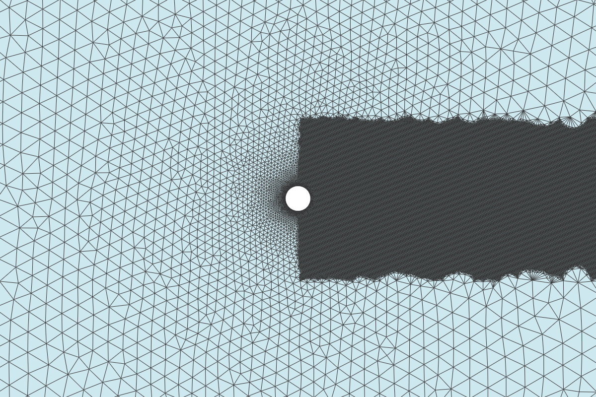
Programmatic mesh generation using gmsh's Python API. Distance-based refinement near the cylinder surface (for boundary layer resolution) combined with a Box field to concentrate cells in the wake region, where vortices form and need the highest resolution.

[C] In [4]: Mesh generator (gmsh)

import gmsh

def cylinder_2d(radius=0.3, farfield_radius=15.0,
                cl_cyl=0.01, cl_far=0.5,
                cl_wake=0.04, wake_length=4.0, wake_width=1.0):
    gmsh.initialize()
    gmsh.model.add("cylinder_2d")

    disk = gmsh.model.occ.addDisk(0, 0, 0, radius, radius)
    farfield = gmsh.model.occ.addDisk(0, 0, 0, farfield_radius, farfield_radius)
    ov, _ = gmsh.model.occ.cut([(2, farfield)], [(2, disk)])
    gmsh.model.occ.synchronize()

    # Distance-based refinement near cylinder
    gmsh.model.mesh.field.add("Distance", 1)
    gmsh.model.mesh.field.setNumbers(1, "NodesList", [surface_tag])
    gmsh.model.mesh.field.add("Threshold", 2)
    gmsh.model.mesh.field.setNumber(2, "InField", 1)
    gmsh.model.mesh.field.setNumber(2, "SizeMin", cl_cyl)
    gmsh.model.mesh.field.setNumber(2, "SizeMax", cl_far)
    gmsh.model.mesh.field.setNumber(2, "DistMin", 0)
    gmsh.model.mesh.field.setNumber(2, "DistMax", radius * 3)

    # Box field for wake refinement
    gmsh.model.mesh.field.add("Box", 3)
    gmsh.model.mesh.field.setNumber(3, "VIn", cl_wake)
    gmsh.model.mesh.field.setNumber(3, "VOut", cl_far)
    gmsh.model.mesh.field.setNumber(3, "XMin", -radius)
    gmsh.model.mesh.field.setNumber(3, "XMax", wake_length)
    gmsh.model.mesh.field.setNumber(3, "YMin", -wake_width)
    gmsh.model.mesh.field.setNumber(3, "YMax", wake_width)

    gmsh.model.mesh.field.add("Min", 4)
    gmsh.model.mesh.field.setNumbers(4, "FieldsList", [2, 3])
    gmsh.model.mesh.field.setAsBackgroundMesh(4)

    cyl_tag = get_physical_tag(gmsh, "wall")
    gmsh.model.addPhysicalGroup(1, [cyl_tag], name="wall")
    gmsh.model.addPhysicalGroup(2, [ov[0][0][1]], name="farfield")

    gmsh.model.mesh.generate(2)
    gmsh.model.mesh.createTopology()  # required for SU2 export
    gmsh.write(f"{name}.su2")
    gmsh.finalize()

Output: SU2 mesh file

Nodes: 44,710 | Triangles: 89,422 | cl@wall: 0.008 | cl@wake: 0.04

4. → Running SU2

[C] In [5]: Execute SU2_CFD

# Run SU2 from the case directory
/Users/ajeet/SU2_CFD/bin/SU2_CFD cylinder.cfg

# Results are written to:
#   history.csv   : convergence of Cl, Cd, residuals
#   flow.vtu      : per-timestep solution (ParaView format)

Terminal output (steady case)

[INFO] SU2 v8.4.0 "Harrier" [INFO] Config file: cylinder.cfg [INFO] Solving INC_RANS with SST turbulence model [INFO] Iteration 500: Cd=0.683 | Cl=-0.032 | RMS_RES=3.2e-06 [...] [INFO] Converged at iteration 3000

5. → Visualization Pipeline (PyVista)

[M] Reading VTU files and rendering frames

PyVista reads the per-timestep VTU files written by SU2 and renders pressure and velocity fields using perceptually uniform colormaps. Each frame is saved as a PNG; imageio stitches them into MP4 animations. Interactive 3D HTML is exported via the trame backend.

[C] In [6]: PyVista frame renderer

import pyvista as pv
import imageio
import numpy as np

def render_frame(vtu_path, field="pressure", cmap="magma",
                 clim=None, camera_pos=None):
    mesh = pv.read(vtu_path)
    plotter = pv.Plotter(off_screen=True, window_size=[1920, 1080])

    if field == "pressure":
        mesh.set_active_scalars("Pressure")
        cmap = "magma"
        title = "Pressure Field"
    else:
        mesh.set_active_scalars("Velocity")
        cmap = "inferno"
        title = "Velocity Magnitude"

    plotter.add_mesh(mesh, cmap=cmap, scalars=mesh.active_scalars_name,
                     clim=clim, show_edges=False)
    plotter.add_title(title)
    plotter.show(auto_close=False)
    img = plotter.screenshot(return_img=True)
    plotter.close()
    return img


# Stitch frames into animation
def make_animation(frame_dir, output_mp4, fps=20):
    writer = imageio.get_writer(output_mp4, fps=fps)
    for f in sorted(frame_dir.glob("*.png")):
        writer.append_data(imageio.imread(f))
    writer.close()

Output: MP4 animation

200 frames @ 20fps = 10s animation | Resolution: 1920×1080

6. → Run Script

[M] Orchestrating the full pipeline

The src/su2_runner.py module provides a high-level API that ties mesh generation, config writing, solver execution, and visualization into a single SU2Solver class.

[C] In [7]: su2_runner.py (key methods)

class SU2Config:
    """Build SU2 .cfg files from Python parameters."""

    def __init__(self, reynolds=40000, length=0.6, magnus=False):
        self.params = {
            "SOLVER": "INC_RANS",
            "KIND_TURB_MODEL": "SST",
            "REYNOLDS_NUMBER": reynolds,
            "REYNOLDS_LENGTH": length,
            "VISCOSITY_MODEL": "CONSTANT_VISCOSITY",
            "MU_CONSTANT": 1.0 / reynolds,
        }
        if magnus:
            self.params.update({
                "SURFACE_MOVEMENT": "MOVING_WALL",
                "MARKER_MOVING": "( wall )",
                "SURFACE_ROTATION_RATE": "0.0 0.0 3.33333",
            })

    def write(self, path):
        with open(path, "w") as f:
            for k, v in self.params.items():
                f.write(f"{k}= {v}\n")


class SU2Solver:
    """Run SU2_CFD and parse results."""

    def __init__(self, binary="/Users/ajeet/SU2_CFD/bin/SU2_CFD"):
        self.binary = binary

    def run(self, case_dir):
        subprocess.run([self.binary], cwd=case_dir, check=True)
        hist = pd.read_csv(f"{case_dir}/history.csv")
        cd = hist["CD"].iloc[-1]
        cl = hist["CL"].iloc[-1]
        return {"Cd": cd, "Cl": cl}