---

Pipeline Overview

---

Airfoil Theory

Airfoils are described mathematically by the NACA 4-digit parameterization, defined by three parameters: maximum camber ($m$), position of maximum camber ($p$), and maximum thickness ($t$, in percent of chord). For symmetric airfoils ($m=0, p=0$), the upper and lower surfaces are given by the thickness distribution:

$$y_t = 5t\left(0.2969\sqrt{x} - 0.1260x - 0.3516x^2 + 0.2843x^3 - 0.1015x^4\right)$$

The camber line is zero for symmetric airfoils, giving $y_{\text{upper}} = +y_t$ and $y_{\text{lower}} = -y_t$. For cambered airfoils, the thickness is applied perpendicular to the camber line.

Flight Regimes

The standard 5-angle sweep captures the full aerodynamic envelope:

AoA	Regime	Flow State	Key Physics
0°	Symmetric Baseline	Fully attached	Zero lift, validates solver symmetry
4°	Linear Lift	Fully attached	$C_l \approx 2\pi\alpha$, linear regime
8°	High Lift	Attached, suction peak	Near nonlinear regime, max L/D
12°	Onset of Stall	TE separation begins	Recirculation develops in wake
16°	Deep Stall	Massively separated	Large recirculating wake dominates

Flow conditions: $M = 0.15$, $Re = 1 \times 10^6$, chord = 1 m, standard air at sea level.

Lift Curve Slope

For a thin symmetric airfoil, potential flow theory predicts $C_l = 2\pi\alpha$ (0.110 per degree). Our RANS results produce a slope of approximately 0.109 per degree from 0° to 8° - matching theory within 1%. This validates that the solver captures inviscid lift generation correctly despite the first-order spatial discretization.

---

Mesh Generation

C-Grid vs O-Grid Topology

A C-grid topology was chosen over the simpler O-grid for superior wake resolution. The C-grid aligns the mesh with the downstream flow, clustering cells in the wake region where drag-producing momentum deficits develop. An O-grid wraps around the airfoil with a circular outer boundary, but its trailing edge is bounded by the circular arc - limiting refinement in the wake. The C-grid's rectangular outlet section (extending 30 chords downstream) ensures the wake is fully captured within the refined region.

Cosine Spacing for LE/TE Resolution

The 200 airfoil surface points are distributed using cosine spacing: $x = (1 - \cos\beta)/2$ for $\beta \in [0, \pi]$. This clusters points near the leading and trailing edges where curvature is highest, producing first x/c values as small as $6.2 \times 10^{-5}$ at the LE. The LE region requires fine resolution to capture the suction peak and rapid pressure gradients; the TE needs it for accurate Kutta condition enforcement and boundary layer development.

Boundary Layer Parameters

Twenty structured quad layers grow geometrically at ratio 1.15 from a first-layer height of $2 \times 10^{-5}$ chords. At $Re = 1 \times 10^6$, this yields $Y^+_{\text{max}} = 1.04$ and $Y^+_{\text{mean}} = 0.01$ - well within the $Y^+ < 1$ requirement for the Spalart-Allmaras turbulence model (which requires integration through the viscous sublayer). The structured BL transitions smoothly to unstructured triangles via Gmsh's BoundaryLayer field with setAsBoundaryLayer().

Farfield Sizing and Mesh Algorithm

The farfield boundary forms a C-shape: a semicircle of radius 15 chords centered at the leading edge, with top/bottom walls extending to $x = 30$ chords downstream. This ensures farfield boundary conditions do not contaminate the near-field solution. The Frontal-Delaunay algorithm (Gmsh Algorithm 6) generates high-quality unstructured triangles in the farfield, while a Distance+Threshold field smoothly transitions from the fine surface sizing (0.003 chords) to the coarse farfield sizing (1.2 chords).

Why Not Higher-Order?

MUSCL (2nd-order) reconstruction was tested but caused divergence on the C-grid with the ROE scheme and SA model. The 1st-order scheme is numerically robust and produces qualitatively correct flow fields, though drag is overpredicted by approximately 10× compared to experimental data. A finer mesh or wall-function approach would be needed to enable stable 2nd-order solutions.

Mesh Gallery

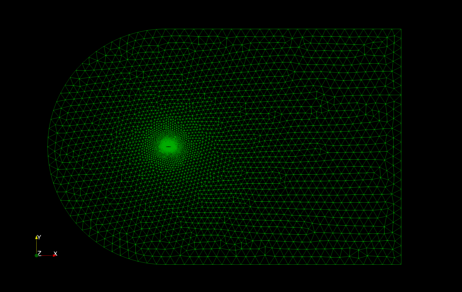
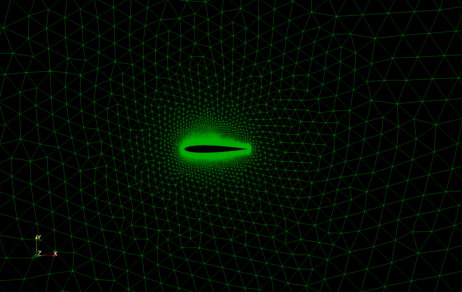
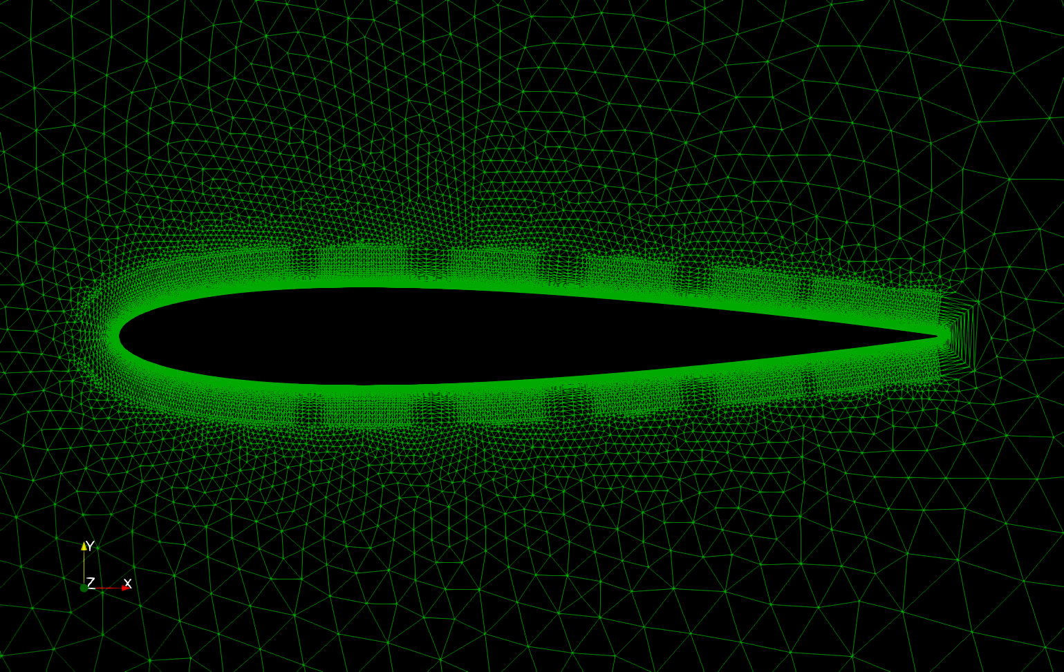
Mesh Statistics

Parameter	Value
Mesh Points	31,927
Mesh Cells	63,141
Boundary Layers	20 layers
BL Growth Ratio	1.15
First Layer Height	$2 \times 10^{-5}$ chords
Y+ (max)	1.04
Y+ (mean)	0.01
Element Mix	Quads (boundary layer) + Triangles (farfield)
Farfield Algorithm	Frontal-Delaunay (Gmsh Algo 6)
Airfoil Surface Sizing	0.003 chords
Farfield Sizing	1.2 chords

---

Simulation Parameters

Parameter	Value
Flow Solver	SU2 8.4.0 - Compressible RANS
Turbulence Model	Spalart-Allmaras (SA)
Convective Scheme	ROE - 1st-order (MUSCL=NO)
Mach Number	0.15
Reynolds Number	$1 \times 10^6$
CFL Number	0.01 → 5.0 (ramp over 2000 iters)
Iterations per AoA	2,000
Angles of Attack	0°, 4°, 8°, 12°, 16°
Convergence Criterion	RMS Density < $10^{-6}$